
Interpretation of Area Under the ROC Curve
Published:
Background
AUROC is one of the most commonly used metric in binary classification tasks. It stands for Area Under Curve - Receiver Operating Characteristics. It is simply the area under the ROC curve. One way of interpreting AUROC is that it is just the area under the ROC curve obtained by interpolating TPR and FPR at different thresholds. There is also another probabilistic interpretation of AUROC. We will state that and prove why that is the case mathematically.
ROC Curve
First, we need to understand the construction of the ROC curve. ROC curve is constructed by finding two metrics (True Positive Rate (TPR) and False Positive Rate (FPR)) at different thresholds.
True Positive Rate (TPR) is simply the recall of the classifier. It is the ratio of number of true positives to the total number of actual positive samples.
\[TPR = \frac{TP}{TP + FN}\]where $TP$ is number of true positives and $FN$ is number of false negatives.
TPR can be interpreted as the ratio of positive samples correctly predicted as positive.
False Positive Rate (FPR) is the ratio of the number of false positives to the total number of actual negative samples.
\[FPR = \frac{FP}{FP + TN}\]where $FP$ = number of false positives and $TN$ = number of true negatives.
FPR can be interpreted as the ratio of negative samples predicted wrongly as positive.
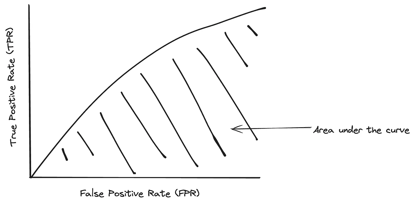
So, the ROC curve has False Positive Rate (FPR) on the X-axis and True Positive Rate (TPR) on the Y-axis.
Mathematics of AUROC
Mathematical Framework
First, let’s formalize the AUROC framework mathematically. Let there be two sets of samples: positive samples and negative samples. $P$ corresponds to the probability distribution of the positive set of samples and $N$ corresponds to the probability distribution of negative set of samples.
Let’s also define $X_p$ and $X_n$ as the random variables that give scores for the randomly chosen positive and negative sample respectively.
The metrics TPR and FPR depend on the threshold value chosen. So, they are functions of the threshold value rather than constants. Let’s define threshold by $k$. Therefore, TPR and FPR are functions of $k$. We represent them by $TPR(k)$ and $FPR(k)$.
Now, the area under the ROC curve is given by the following integral:
\[\int_{0}^{1} TPR(k) \, d(FPR(k))\]TPR for the threshold $k$, $TPR(k)$, is given by the probability that the random variable $X_p$ is greater than the threshold $k$ i.e., $TPR(k) = P(X_p > k)$.
The cumulative distribution function for the random variable $X_p$ can be defined as: \(F_{X_p}(k) = P(X_p < k)\)
So, $TPR(k) = P(X_p > k) = 1 - P(X_p \leq k) = 1 - F_{X_p}(k)$
Similarly, FPR for the threshold $k$, $FPR(k)$, is given by the probability that the random variable $X_n$ is greater than the threshold $k$ i.e., $FPR(k) = P(X_n > k)$.
The cumulative distribution function for the random variable $X_n$ can be defined as: \(F_{X_n}(k) = P(X_n < k)\)
So, $FPR(k) = P(X_n > k) = 1 - P(X_n \leq k) = 1 - F_{X_n}(k)$
Now, the integral reduces to:
\[\text{AUROC} = \int_{0}^{1} (1 - F_{X_p}(k)) \, d(1 - F_{X_n}(k))\]Let $z = 1 - F_{X_n}(k)$.
Then, $dz = -f_{X_n}(k)dk$.
The limits go from $+\infty$ to $-\infty$. So, the integral with change of variables and limits becomes:
\[\text{AUROC} = \int_{0}^{1} (1 - F_{X_p}(k)) \, dz\] \[\text{AUROC} = -\int_{+\infty}^{-\infty} (1 - F_{X_p}(k)) f_{X_n}(k) \, dk\]Swapping the integral limits,
\[\text{AUROC} = \int_{-\infty}^{+\infty} (1 - F_{X_p}(k)) f_{X_n}(k) \, dk\]Now, expanding the integration,
\[\text{AUROC} = \int_{-\infty}^{+\infty} f_{X_n}(k) \, dk - \int_{-\infty}^{+\infty} F_{X_p}(k) f_{X_n}(k) \, dk\]The first term is area under the probability density function $f_{X_n}$. The total area under any probability density function is 1.
\[\text{AUROC} = 1 - \int_{-\infty}^{+\infty} F_{X_p}(k) f_{X_n}(k) \, dk\]Here, the integral term in the right can be interpreted as the expectation of the term $F_{X_p}$ over the probability density function $f_{X_n}$. This is essentially expectation of random variable $F_{X_p}$ over the random variable $X_n$. So, the area under the curve can be written as:
\[\text{AUROC} = 1 - \mathbb{E}_{X_n \sim N} [F_{X_p}(X_n)]\]Please note that $N$ is the probability distribution of scores for negative samples. The cumulative distribution function, $F_{X_p}$, can be written as:
\[\text{AUROC} = 1 - \mathbb{E}_{X_n \sim N} [P(X_p < X_n)]\]The probability, $P(X_p < X_n)$, of two random variables $X_p$ and $X_n$, is a number. So, the expectation turns out to be the probability itself. Hence:
\[\text{AUROC} = 1 - P(X_p < X_n) = P(X_p > X_n)\]So, we showed how AUROC is just the probability that the score coming from random positive sample is greater than the score coming from random negative sample.
Final Thoughts
Therefore, AUROC can be an excellent measure of how the model/system can distinguish positive and negative samples. If the model always ranks all the positive samples above all the negative samples, the AUROC would be 1. This interpretation also clarifies why AUROC of 0.5 is the worst. A model can give completely random values to the samples and there would always be 50% probability the the score coming from positive sample is higher than the score coming from negative sample.